What this project is
This project builds a decentralized search and rescue system. Two quadruped robots operate in a simulated world. The robots must find a target that moves. No central computer controls the robots. Each robot has its own sensors, its own memory, and its own decisions. The robots exchange messages over a network protocol.
The project has seven phases. Each phase adds one capability. Each phase also teaches one concept that transfers to other robot platforms, such as drones or boats.
Robot names The first robot has the name Walnut. The second robot has the name Hazel.
The phases
The system running
These two recordings show the Phase 4b forest run. The arena is 11 m × 11 m and contains 18 tree obstacles. Walnut and Hazel search independently. The red sphere is the target, which follows a Lissajous figure-eight path. The thin green and red lines are the infrared rays from the sensor ring of each robot.
Neither robot knows where the target is at the start. Neither robot can read the memory of the other robot. All coordination happens through the UDP messages described in Phase 3.
Forest run 1 — both robots search. The two quadrupeds start near the centre and move outward through the trees. Watch the infrared rays change colour as they meet a trunk. The artificial potential field keeps each robot clear of the trunks and clear of the other robot.
Forest run 2 — approach to the target. One robot moves close to the red sphere. The camera then pulls back to show the full arena. The target continues to move along its figure-eight path, so the robots must keep tracking it rather than stop at one position.
The simulated world
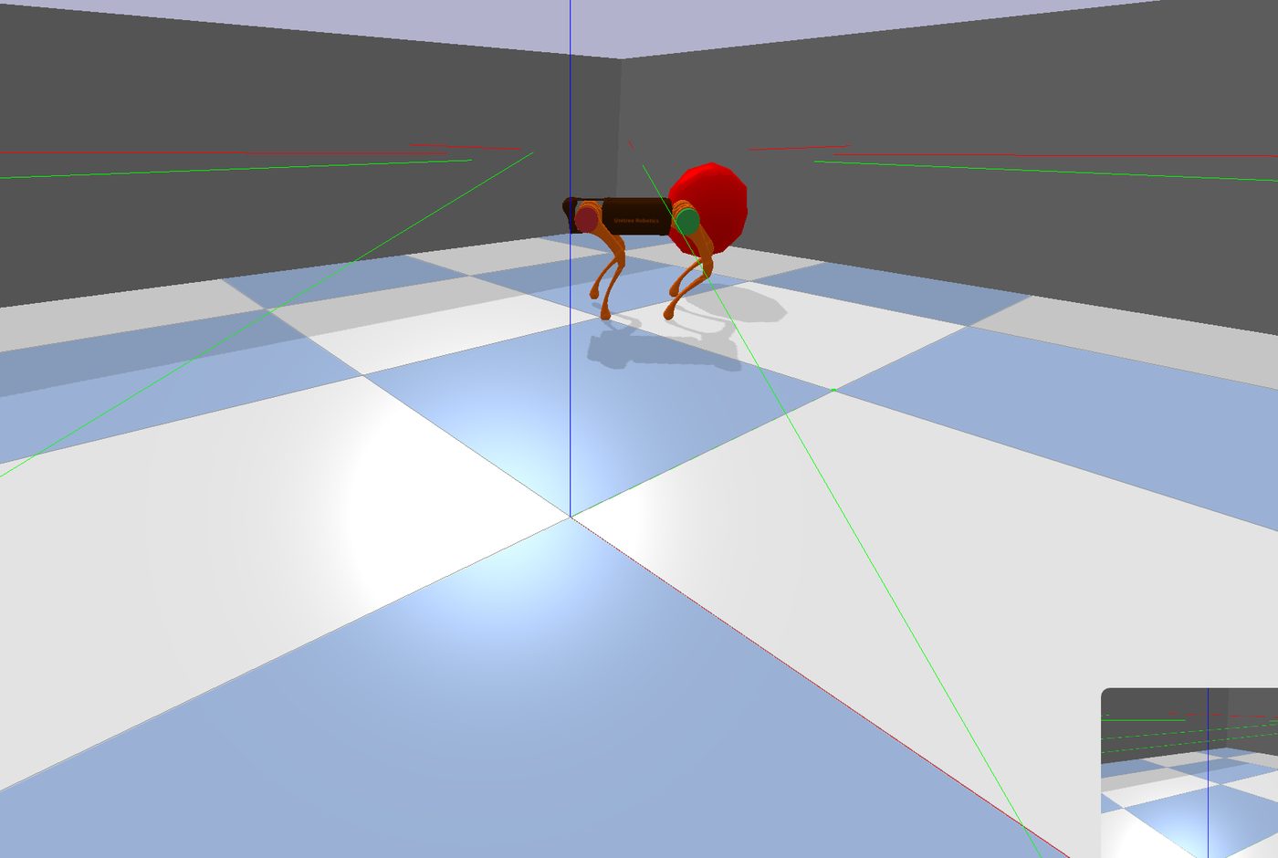 One robot, empty arenaThe early configuration. The green and red lines are the eight infrared rays from the sensor ring.
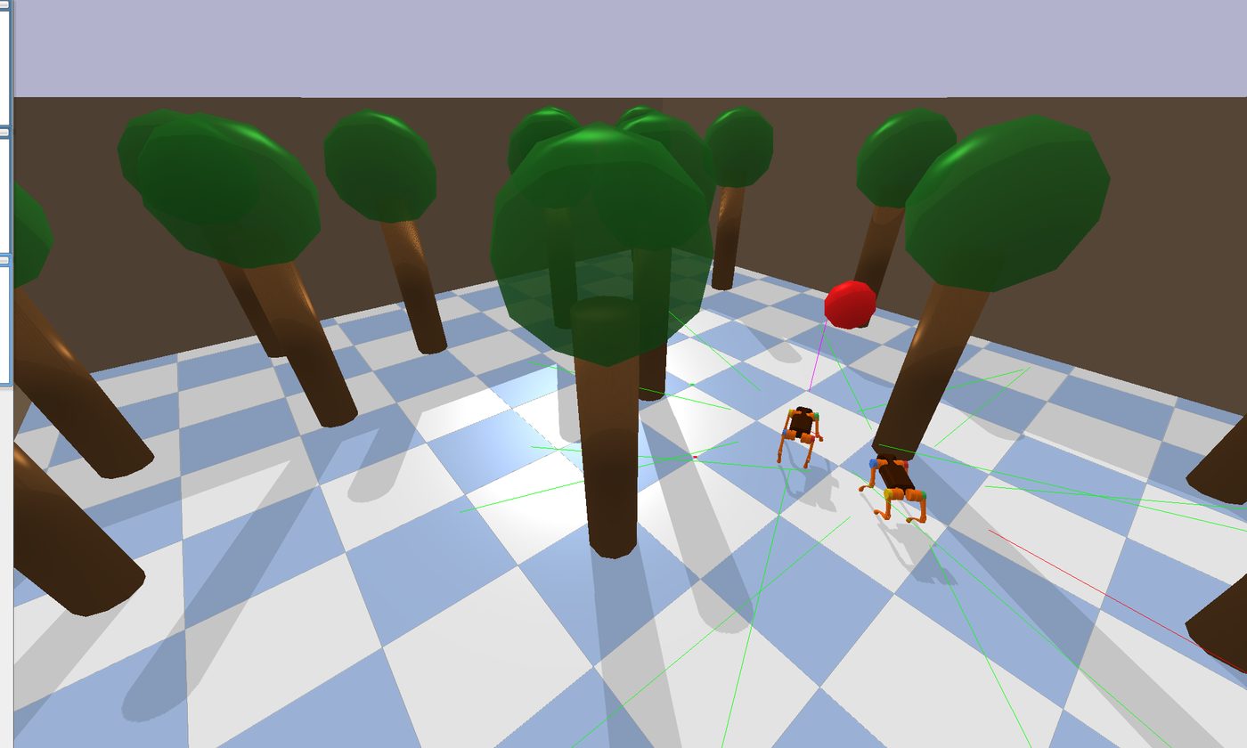 Walnut and Hazel in the forestBoth robots operate in the same physics world, as separate processes connected to a PyBullet server.
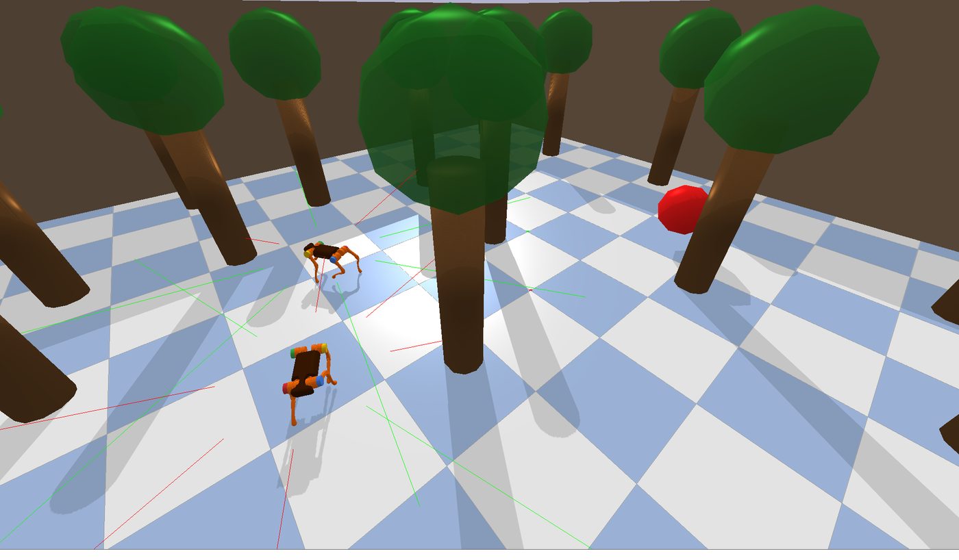 Close view of the sensor raysGreen means the ray met nothing within range. Red means the ray met a trunk or a wall.
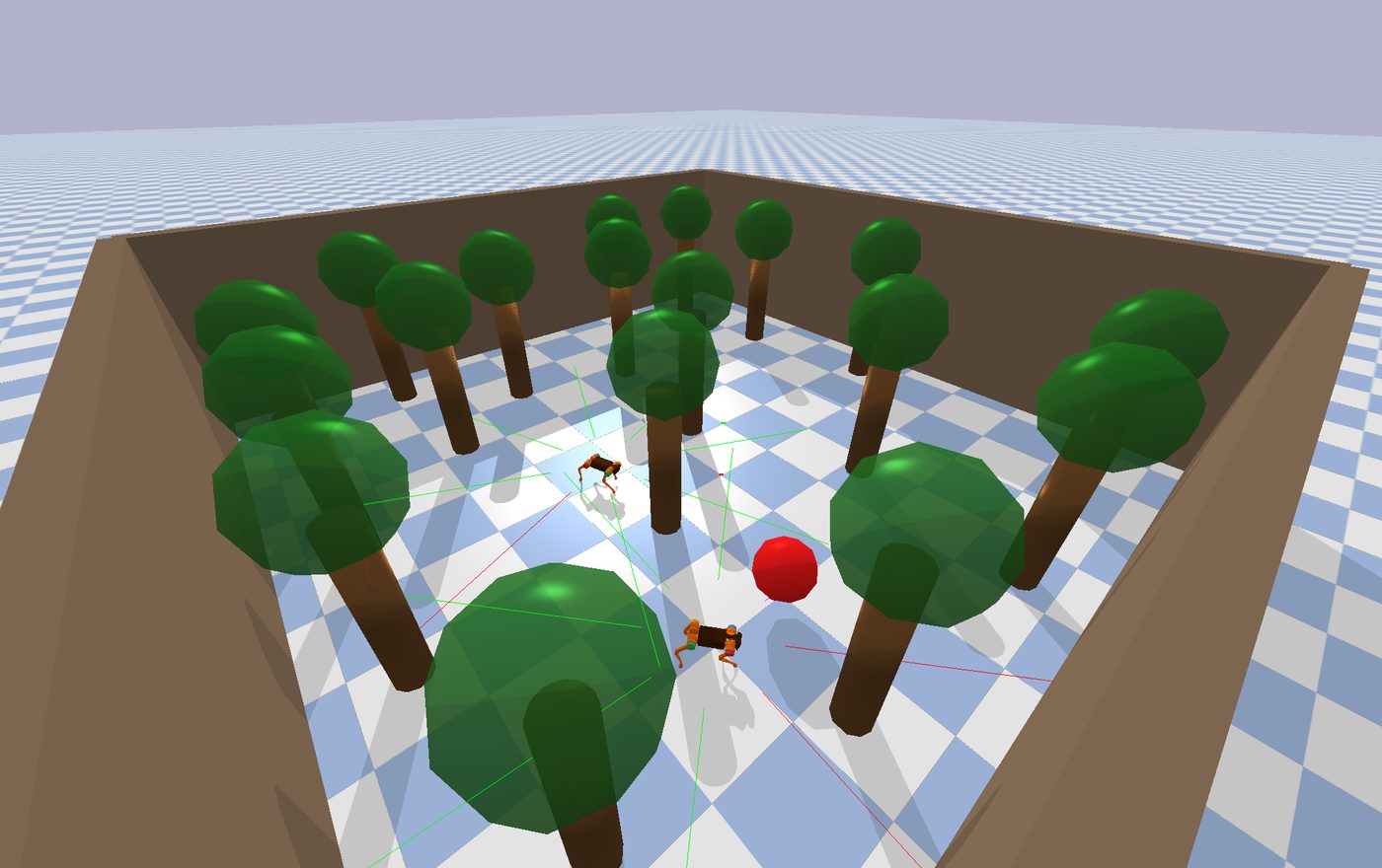 The full arena11 m × 11 m, four walls, and 18 trees at 1.8 m spacing. The spacing lets a robot pass between any two trunks.
Results at a glance
Each phase produced measured results. Select a plot to open the phase that explains it.
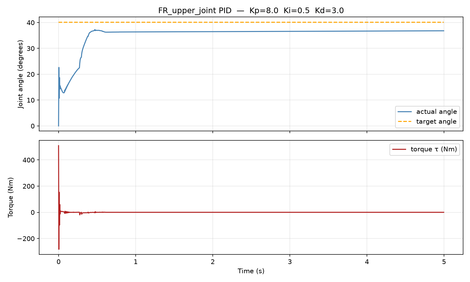 Phase 1A — tuned PID jointKp = 8.0, Ki = 0.5, Kd = 3.0. The torque settles near zero, because the gravity feedforward term carries the static load.
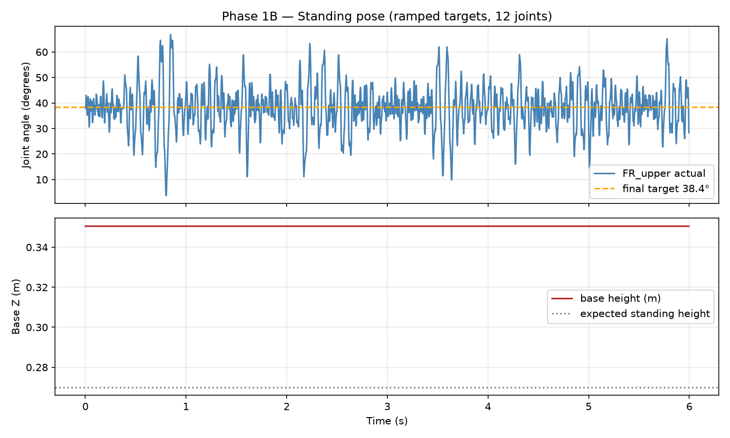 Phase 1B — standing pose, 12 jointsThe flat base height line confirms that the body is fixed. The joint oscillation comes from ground contact.
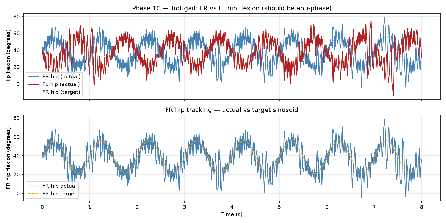 Phase 1C — trot gait at 1 HzThe front-right hip and the front-left hip are in anti-phase. This is the trot pattern.
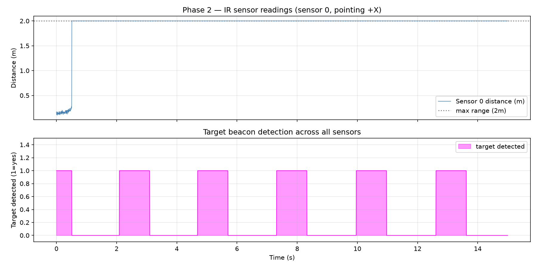 Phase 2 — infrared sensor arraySix detection pulses, one for each pass of the target across a sensor ray.
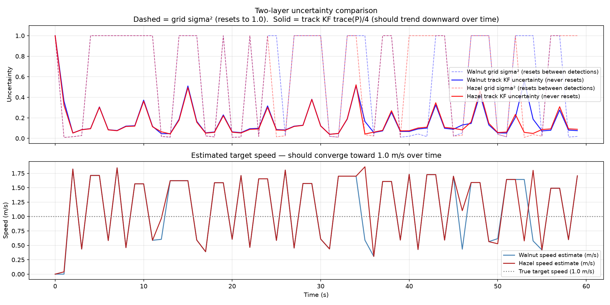 Phase 3 — the two filter layersThe dashed grid traces reset to 1.0. The solid track traces never reset. That separation is what Layer 2 adds.
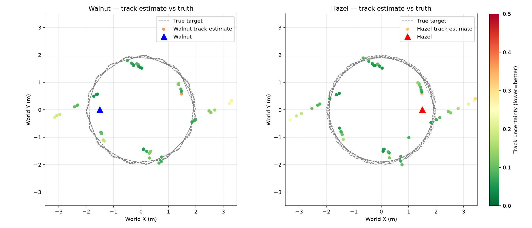 Phase 3 — track estimate against truthDark green means low uncertainty. Both robots track the target accurately from opposite sides of the arena.
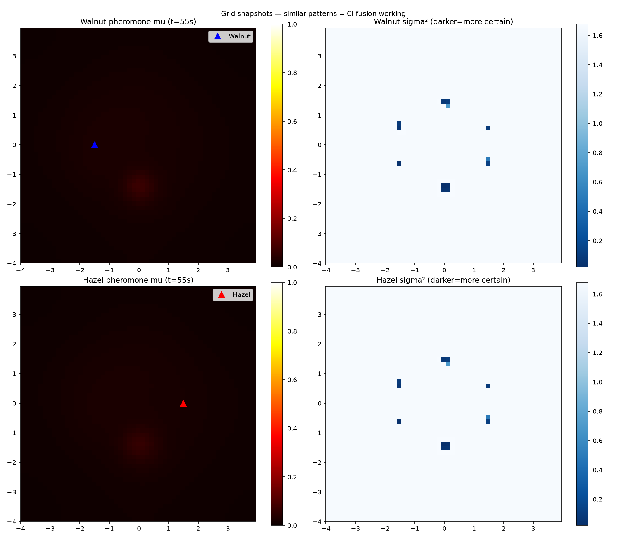 Phase 3 — covariance intersection, visibleThe confident cells sit at the same world positions in both grids, although the robots share no memory.
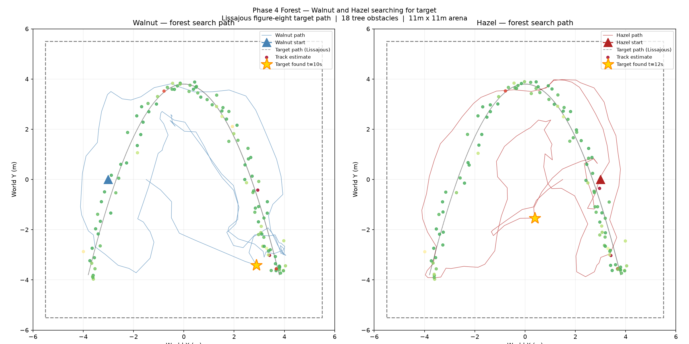 Phase 4 — search in a forest18 obstacles, an 11 m × 11 m arena, and a figure-eight target path. Walnut found the target at t = 10 s, Hazel at t = 12 s.
The full plan
Phase 0 — Setup and the dynamics (about 3 hours)
Install PyBullet. Load a quadruped URDF model. Let the model stand under gravity. Learn the rigid-body equation:
\[M(q)\,\ddot{q} + C(q,\dot{q})\,\dot{q} + g(q) = \tau\]Learn what each term means. Learn why the simulator solves this equation at each timestep. Examine the URDF file. Identify the links and the joints. Learn what “state” means. The state is the joint angles, the joint velocities, the base pose, and the base twist. Do not write a controller in this phase. First understand what you will control.
Phase 1 — Single-robot control and locomotion (about 9 hours)
Write a joint PID position controller. Tune one joint. Observe the overshoot. Observe the steady-state error. Learn the effect of each gain.
Then build a gait generator. The gait generator uses foot trajectories with parameters. Each leg has a different phase offset. A trot gait moves the diagonal legs together.
Locomotion has two parts. The first part is trajectory generation, which decides where the feet must go. The second part is tracking, which is the PID controller that moves the joints to the necessary positions. This structure is a cascade. A drone uses the same structure: position, then attitude, then motor.
Also write an LQR controller for a cart-pole system. The cart-pole has less complexity than the quadruped. This makes optimal model-based control easier to learn.
The cascade structure and the difference between PID and LQR apply to all robot platforms.
Phase 2 — Perception (about 6 hours)
Simulate infrared sensors with ray casts from the robot body. Use the rayTest
function. Real infrared sensors and lidar sensors work in the same way: they send a
ray and they measure the distance to the first object.
Add a field of view. Add Gaussian noise, because real sensors are not exact.
Give the target an infrared beacon. The sensor must identify this beacon. The sensor returns the bearing and the range when the beacon is in view.
Learn the difference between three operations:
- Detection — is an object present?
- Localization — where is the object, and in which frame?
- Recognition — what is the object?
Also learn the coordinate transforms from the sensor frame to the body frame, and from the body frame to the world frame.
The same sensor model becomes obstacle detection on a drone, or sonar on a boat.
Phase 3 — The decentralized communication protocol (about 9 hours)
This phase is the most important part of the project.
Divide the system into two independent agent processes. Design a message schema. Start with JSON:
{ "robot_id": "walnut", "timestamp": 12.4, "position": [1.2, 0.8],
  "heading": 0.35, "detections": [], "help_request": null }
Send the messages over UDP. Then add shared-belief fusion. Each agent adds the detections of the other agents to its own world model. Handle messages that are late or lost. Use timestamps and timeouts.
Learn the difference between centralized systems and decentralized systems. Learn protocol design. Learn why local-only knowledge is the core problem.
This layer transfers without change to drones and boats. It is the most expandable part of the project.
Phase 4 — Collision avoidance and search strategy (about 6 hours)
Write artificial potential fields. An attractive force pulls the robot to the target. A repulsive force pushes the robot away from obstacles and away from the other robot.
The robot will stop in a local minimum. This failure is part of the lesson. It shows why engineers use Velocity Obstacles or ORCA instead.
For the search problem, divide the arena between the two robots. This is distributed area partitioning. Then run a lawnmower sweep pattern.
Learn the difference between reactive methods and deliberative methods. Learn the limits of purely local methods.
Phase 5 — Integrate, scale, and measure (about 5 hours)
Run the full mission. Both robots search. One robot finds the target. That robot calls the other robot. Both robots move to the target. The robots do not collide.
Then start three or four agent processes. If the Phase 3 design is correct, this works without new code. This result proves that decentralization scales.
The communication volume increases as O(n²). Add range-limited messaging to correct this.
Measure the time to find the target, the number of collisions, and the messages per second.
Learn about emergence and about the trade-offs of scale.
Phase 6 — The hardware test (optional, about 3 hours)
Use one ESP32 microcontroller (approximately $8), one infrared sensor (approximately $2), and a breadboard. Connect the components. Read the sensor in code. Then make the ESP32 send a real UDP message into the simulated swarm.
This is a simulation-to-reality bridge. A physical sensor changes the behaviour of virtual agents. This method has the name hardware-in-the-loop.
Repository layout
swarm_robotics/
├── phase1/
│   ├── pid_control.py          # Phase 1A — single joint PID
│   ├── standing.py             # Phase 1B — 12-joint standing pose
│   ├── gait_generator.py       # Phase 1C — trot gait
│   └── plot_gait.py
├── phase2/
│   ├── ir_sensor.py            # IRSensor and IRSensorArray classes
│   └── plot_sensor.py
├── phase3/
│   ├── pheromone_grid.py       # per-cell Kalman filter grid
│   └── plot_phase3.py
├── phase4/
│   ├── navigators.py           # Frontier, APF, Waypoint
│   └── phase4_forest.py
└── docs/                       # this site (GitHub Pages)
How to read these pages
Each phase page is divided into tabs. The tab bar stays at the top of the page while you scroll. Select a tab to replace the content below it. Use the previous and next controls at the foot of each tab to move through a phase in order.
The theme control is at the foot of the sidebar. It has three states: system, light, and dark. The system state follows your operating system setting.
A note on the writing
These pages use ASD-STE100 Simplified Technical English. This standard uses short sentences, the active voice, and one meaning for each word. The standard removes idioms and metaphors. The purpose is clear technical communication.
Some sentences keep a comparison, such as the comparison to ant colonies. These comparisons are necessary to explain the concept. They are written as plain statements.