Goal
Answer this question: how do you make a robot body do what you tell it to do?
Phase 1 has three parts:
| Part | Subject | Result |
|---|---|---|
| Phase 1A | Single-joint PID control | One tuned joint that holds a commanded angle |
| Phase 1B | Standing pose | Twelve controllers hold a configuration against gravity |
| Phase 1C | Trot gait | Each joint follows a trajectory instead of a constant |
Command reference
These commands were necessary during the phase.
| Command | Function |
|---|---|
code . |
Open the current folder in VS Code from the terminal |
exit |
Leave the WSL terminal |
wsl --shutdown |
Shut down WSL |
nvidia-smi |
Show whether the GPUs are available and operational |
explorer.exe <path> |
Open a file, such as a PNG plot or a PDF, in Windows |
touch <path> |
Create an empty file at the given path |
cat <path> |
Print the contents of a file |
cp <source> <target> |
Copy a file from the source path to the target path |
head -3 <path> |
Print the first three lines of a file |
source ~/venv/bin/activate |
Activate the Python virtual environment |
Phase 1A — Single-joint PID control
What a PID controller is
PID means Proportional-Integral-Derivative. A PID controller is a feedback control mechanism. The controller calculates an error value continuously. The error is the difference between the desired setpoint and the current state. The current state also has the name measured process variable. The controller then makes corrections. The corrections make the system stable and accurate.
\[\tau = K_p e + K_i \int e\,dt + K_d \dot{e}\]The steady-state error
The first test used $K_i = 0$. The logs show the result.
  t=0.0s  angle=+0.0000 rad  error=+0.7000  tau=+182.000 Nm
  t=0.5s  angle=+0.7849 rad  error=-0.0849  tau=+0.501 Nm
  t=1.0s  angle=+0.7613 rad  error=-0.0613  tau=-1.227 Nm
  t=1.5s  angle=+0.7612 rad  error=-0.0612  tau=-1.224 Nm
  t=2.0s  angle=+0.7610 rad  error=-0.0610  tau=-1.221 Nm
  t=2.5s  angle=+0.7608 rad  error=-0.0608  tau=-1.215 Nm
  t=3.0s  angle=+0.7605 rad  error=-0.0605  tau=-1.210 Nm
  t=3.5s  angle=+0.7602 rad  error=-0.0602  tau=-1.204 Nm
  t=4.0s  angle=+0.7599 rad  error=-0.0599  tau=-1.200 Nm
  t=4.5s  angle=+0.7596 rad  error=-0.0596  tau=-1.177 Nm
After $t = 0.5\ \text{s}$, the angle and the error stay near the same values. The error does not go to zero. This remaining error has the name steady-state error.
Gravity causes the steady-state error. Gravity is a constant external disturbance. In a system without integral control, the actuator must produce an opposing force. This force holds the position against gravity.
The core problem The joint holds a leg segment against gravity. Gravity pulls the leg down with a constant torque. Call this torque $\tau_{\text{gravity}}$. To hold the leg exactly at the target angle, the controller must produce exactly $\tau_{\text{gravity}}$ in the upward direction. It must not produce more torque. It must not produce less torque.
Why the proportional term alone cannot remove the error
The proportional term is:
\[\tau = K_p \cdot e\]The joint is at 0.76 rad. The target is 0.70 rad. The error is therefore −0.06 rad. With $K_p = 20.0$:
\[\tau = 20.0 \times (-0.06) = -1.2\ \text{Nm}\]This −1.2 Nm opposes gravity at that position. The joint stops there because −1.2 Nm is the exact torque that balances gravity at that angle.
This causes a problem. The proportional term produces more torque only if the error increases. The error increases only if the joint moves further from the target. So a pure proportional controller can produce sufficient torque only at a position that is incorrect. The incorrect position is the source of the torque. The error and the gravity load reach an equilibrium. The joint stays at that point permanently.
Two methods remove this error:
- Use a very high $K_p$. This method causes oscillation. If you increase the error magnitude, the system tries to correct the error continuously. The system then oscillates between the states. To increase the error, the joint must move further from the target. This also increases the position error.
- Add a term that produces torque without an error. The integral term does this. The feedforward term also does this.
How the integral term works
The integral term is:
\[\tau_{\text{integral}} = K_i \int e\,dt \approx K_i \sum (e \cdot dt)\]At each timestep with a nonzero error, the controller adds a small amount to a running total. Over time, even a small constant error becomes a large total. That total produces torque even when the current error is small.
The integrator has one important property. The integrator increases while an error exists. The integrator stops only when the error is exactly zero. Therefore the integrator continues to push the joint until the joint reaches the target. The integrator cannot stop before the error is zero.
With $K_i = 0$, the integral term contributes nothing. The running total increases, but the controller multiplies the total by zero. The proportional term reaches its gravity-balance equilibrium at 0.76 rad. The joint then stays there. No force moves the joint the last 0.06 rad.
With a small value such as $K_i = 0.5$, the result is different:
t=1.0s:  integral ≈ 0.06 × 1.0s = 0.06  →  tau_integral = 0.5 × 0.06 = 0.03 Nm  (small)
t=2.0s:  integral ≈ 0.06 × 2.0s = 0.12  →  tau_integral = 0.5 × 0.12 = 0.06 Nm
t=5.0s:  integral ≈ 0.06 × 5.0s = 0.30  →  tau_integral = 0.5 × 0.30 = 0.15 Nm  (significant)
This increasing term adds to the proportional torque. It moves the joint the remaining distance to the target. The error then becomes zero. The integrator stops. The joint holds position without any error, because the integrator stores the gravity-compensation torque.
Why feedforward is better than the integral term for gravity
The integral term operates correctly, but it has one side effect. The side effect has the name integral windup.
If an obstacle stops the joint before the target, the integrator continues to increase. It has no limit. The integrator stores a very large torque. When the obstacle moves away, the joint receives all of that stored torque at once. Real robots have broken their own joints in this way.
Gravity feedforward is the better method. Compute $\tau_{\text{gravity}}$ analytically from the robot configuration. Use the $g(q)$ term from the manipulator equation in Phase 0. Then add the result directly to the PID output:
\[\tau = K_p e + K_i \int e\,dt + K_d \dot{e} + g(q)\]The PID controller now handles only the dynamic error. The controller never has to oppose gravity, because you compensate gravity explicitly.
PyBullet computes $g(q)$ with the function calculateInverseDynamics().
This method is necessary in Phase 1B. There, twelve joints hold a standing pose at the same time. To oppose gravity on twelve joints with $K_i$ alone would cause windup on all of them.
The three tuning conditions
| Condition | Behaviour | Cause |
|---|---|---|
| Overdamped | The angle moves slowly toward the target. It never reaches the target. | $K_p$ is too low for the gravity load |
| Underdamped | The angle passes the target. It oscillates. Then it stops. | $K_d$ is too low for the value of $K_p$ |
| Well tuned | The angle increases quickly. The overshoot is small or absent. The angle stops at the target. | Correct balance of all three gains |
The tuning procedure
Change one variable at a time.
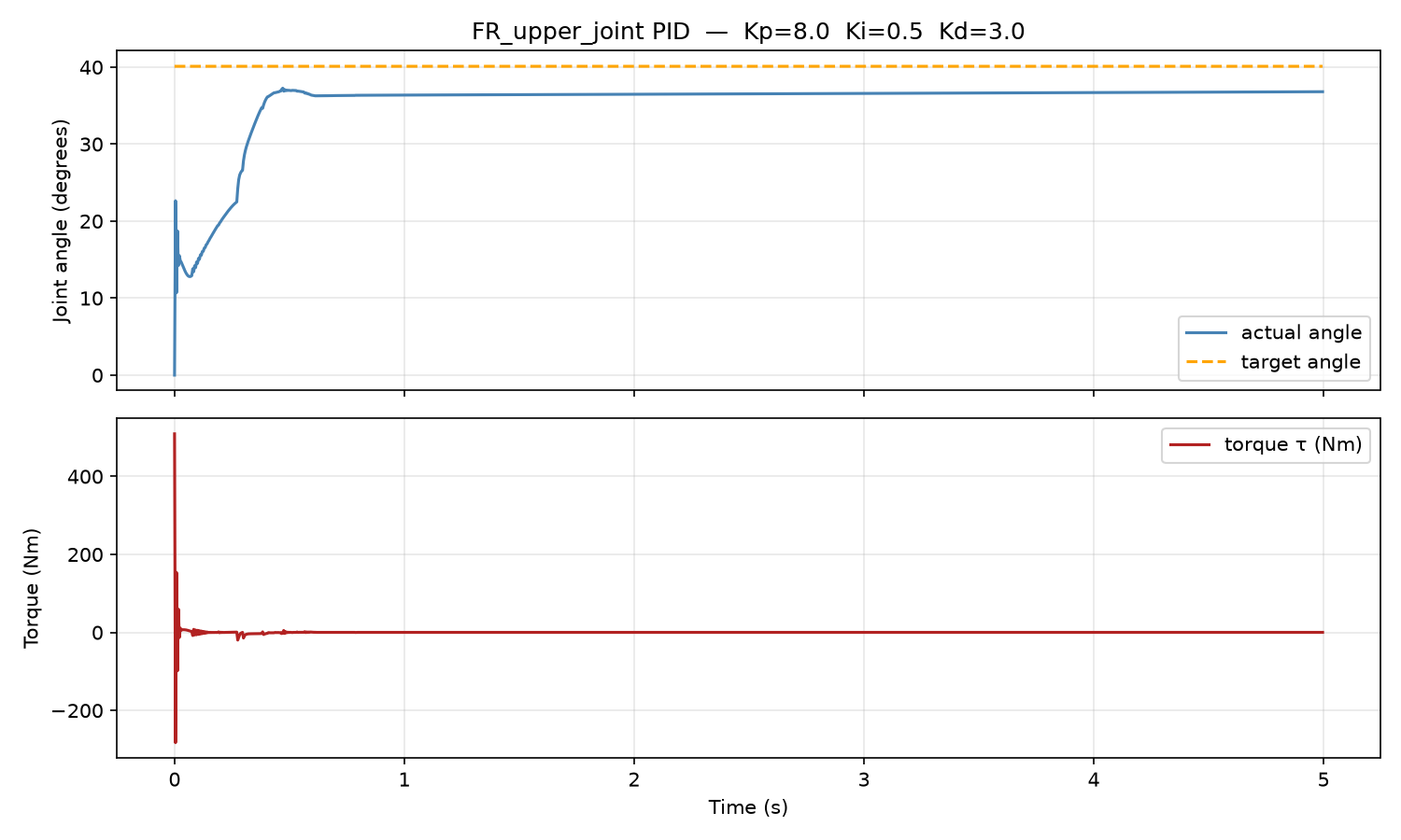
- Reduce $K_p$ from 20.0 to 8.0. A large overshoot occurred. A lower proportional magnitude prevents that overshoot. Note the trade-off: less proportional force means that gravity moves the leg closer to the ground.
- Increase $K_d$ from 1.0 to 3.0. This makes the error converge in the correct direction, toward the target angle. It also reduces the initial overshoot.
- Increase $K_i$ from 0 to 0.5. This moves the steady-state error toward zero.
At this point the torque comes only from the P, I, and D terms. These three terms do all of the work. They oppose gravity and they track the target angle at the same time. The integral term does most of the gravity compensation.
Gravity feedforward separates the two functions:
\[\tau_{\text{total}} = \tau_{\text{PID}} + \tau_{\text{gravity}}\]The result is a working PID controller with gravity feedforward.
PyBullet note
The POSITION_CONTROL mode in PyBullet applies this internally:
This is a PD controller. It has no integral term.
Phase 1B — Standing pose
Goal
Scale Phase 1A to twelve joints, and therefore twelve controllers. The system must hold a desired configuration against gravity on a multi-joint system.
The balance problem
Several difficulties occurred. The robot did not stay in a standing position. It rolled over. Every time the joints started to move, the robot rolled over in some way.
Two corrections were attempted:
- A wider stance. All hip abductors received outward angles instead of 0 degrees. This did not correct the problem.
- Stiffer hip abductors. $K_p$ and $K_d$ were increased for the hip abductors. This also did not correct the problem.
Conclusion PID control and balance are two separate problems. A correct joint controller does not give you a balanced robot.
The solution was the option useFixedBase=True. This option attaches the robot body to
the world. Only the joints then move. This makes gait generation and joint coordination
possible without a balance problem.
This identified a new problem area: free-floating balance. Boston Dynamics used several years to solve this problem. The balance problem stays unsolved in this project.
Result
Kp=20.0  Kd=2.0  maxForce=33.0

  t=0.0s  FR_upper=38.4deg  target=38.4deg  error=-0.0deg
  t=1.0s  FR_upper=43.7deg  target=38.4deg  error=-5.3deg
  t=2.0s  FR_upper=45.3deg  target=38.4deg  error=-6.9deg
  t=3.0s  FR_upper=44.2deg  target=38.4deg  error=-5.8deg
  t=4.0s  FR_upper=37.3deg  target=38.4deg  error=1.1deg
  t=5.0s  FR_upper=32.3deg  target=38.4deg  error=6.1deg
The roll problem is corrected. However, the robot does not move to a new position. Its legs move in a fixed position.
This behaviour is correct and expected. The base height plot is a flat line at 0.35 m for all six seconds. The body is attached to the world. The joints oscillate by about ±5 degrees around the target. Ground contact forces cause these small disturbances. This is normal and acceptable.
Phase 1B is a standing task, not a walking task. The legs hold a static pose against gravity. The only motion is the reaction of the joints to ground contact disturbances. This is realistic physics.
The oscillation in the joint angle plot is ±5 to 7 degrees around 38.4 degrees. This is slightly more noise than ideal. The cause is a $K_d$ value of 2.0, which is a little too low. The result is sufficient to continue. No more tuning was done.
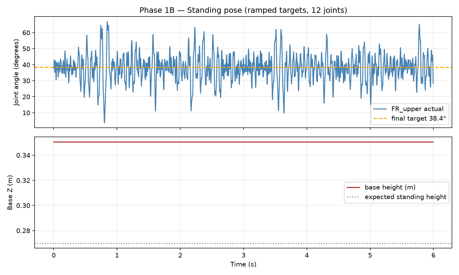
useFixedBase=True holds the body. The dotted line shows the expected standing height.Phase 1C — The trot gait
The conceptual change
The change from Phase 1B to Phase 1C is one idea. The target angles are no longer constants. The target angles are now functions of time.
Phase 1B used a standing_angles dictionary that mapped each joint to one value. This
dictionary now becomes a function. The function returns different values at each
timestep, based on a gait cycle. That function is the gait generator.
The PD controller code does not change between Phase 1B and Phase 1C.
How the gait generator works
A quadruped gait generator computes joint positions, which are angles, as a function of time. The robot walks when two conditions are true:
- Each joint alternates between a stance state and a swing state.
- Phase coordination exists. The front-right leg and the rear-left leg operate together. The front-left leg and the rear-right leg also operate together.
When the robot walks, the hip flexion joint of each leg swings in the direction of travel. The knee joint moves up or down. This produces the lift. These two motions produce the stance state and the swing state.
For quadruped phase coordination, the two diagonal pairs move in anti-phase. The phase offset is $\pi$. If the front-right and rear-left legs are at phase $\pi$, then the front-left and rear-right legs are at phase $2\pi$. Use this relation to calculate the phase at each timestep.
The hip abductor joint does not move.
Any noise in the movement comes from ground contact.
Commands
touch phase1/gait_generator.py
code phase1/gait_generator.py

cp /mnt/c/Users/ankit/Downloads/gait_generator.py ~/projects/swarm_robotics/phase1/gait_generator.py
cp /mnt/c/Users/ankit/Downloads/plot_gait.py ~/projects/swarm_robotics/phase1/plot_gait.py

python3 phase1/gait_generator.py
python3 phase1/plot_gait.py
explorer.exe phase1/gait_result.png
What to observe
In the graphical interface. The body stays fixed, because useFixedBase=True. The
four legs step in a trot pattern. The front-right leg and the rear-left leg move forward
together. At the same time, the front-left leg and the rear-right leg swing back. Then
the pattern reverses. The gait comes from the sinusoidal target functions.
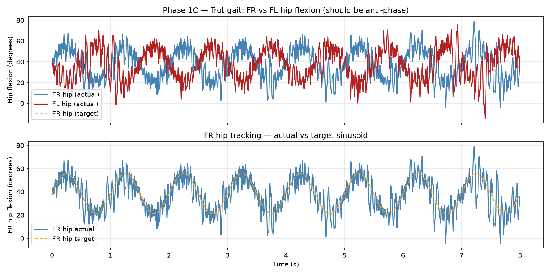
In the plot. The front-right hip and the front-left hip must be mirror images. When the front-right hip is at its forward peak, the front-left hip must be at its backward peak. This anti-phase relation is the trot.
Result
Running trot gait — freq=1.0Hz  swing=0.3rad  lift=0.2rad
Kp=20.0  Kd=2.0  maxForce=33.0
  t=0.0s  FR_hip=38.4deg  FL_hip=38.4deg  (should be anti-phase)
  t=1.0s  FR_hip=25.7deg  FL_hip=12.0deg  (should be anti-phase)
  t=2.0s  FR_hip=27.5deg  FL_hip=42.7deg  (should be anti-phase)
  t=3.0s  FR_hip=32.3deg  FL_hip=50.2deg  (should be anti-phase)
  t=4.0s  FR_hip=39.9deg  FL_hip=35.8deg  (should be anti-phase)
  t=5.0s  FR_hip=36.6deg  FL_hip=36.7deg  (should be anti-phase)
  t=6.0s  FR_hip=37.8deg  FL_hip=40.8deg  (should be anti-phase)
  t=7.0s  FR_hip=42.4deg  FL_hip=39.7deg  (should be anti-phase)
Observation during the run. The gait operates, but the legs move too quickly for an accurate visual assessment.
Assessment. This is a good result. In the lower plot, the front-right hip tracks the orange sinusoidal target correctly. The gait generator operates. The noise on the sinusoid comes from ground contact forces on the joints. This is physically correct.
The upper plot shows that the front-right hip in blue and the front-left hip in red are in anti-phase. When the front-right hip is at a peak, the front-left hip is near its minimum. This is the trot pattern. The result is not clean, because the gains are not tight enough for exact tracking. But the phase relation is present.
The quick leg motion is a display artifact. The cause is time.sleep(DT * 2). This makes
the simulation run at twice real time on screen. Change the value to time.sleep(DT * 8)
to see the gait in slow motion.
Phase 1 summary
Phase 1A established the basic unit. This was a single-joint PID controller with manual tuning. Gravity feedforward separated disturbance rejection from the tracking task.
Phase 1B scaled that unit to twelve simultaneous joints. The joints held a fixed configuration. This proved that joint coordination operates correctly.
Phase 1C replaced the constant targets with time-varying sinusoidal targets. The result was a trot gait at 1 Hz. The front-right and front-left hips were in anti-phase. The legs stepped in diagonal pairs.
The PD controller code did not change between Phase 1B and Phase 1C. This proves that the cascade architecture is correct. The gait generator is only a target-angle function. It is completely separate from the method that executes those angles.
Next
Phase 2 gives the robot sensors. Continue to Phase 2 — Perception.