Phase 4 — Navigation and Search — Swarm Robotics

Goal

The robots must now navigate an unknown environment to find a target. Two problems occur immediately.

Problem 1 — collision. The robots can collide with objects, with walls, and with each other.

Problem 2 — search strategy. In an unknown environment, in which direction do you travel? Collision avoidance and search strategy are both necessary.

Artificial potential fields

The system avoids collisions with artificial potential fields (APF).

The method treats the robot as a particle in a force field. Obstacles apply a repulsive force. This net force pushes the robot away from the obstacles.

Frontier-based coverage

Each robot keeps a list of unexplored regions. This list is the frontier. The robot takes the list from its own pheromone grid. The robot then moves to the nearest unexplored frontier.

A frontier cell has two properties:

Its $\mu$ value is below a threshold.
Its variance is high.

This method distributes the two robots without an explicit rule. When Walnut moves to a frontier, his grid updates travel to Hazel through covariance intersection fusion. The frontier list of Hazel then updates. It removes that region from the search.

Problems and corrections

The locomotion problem

The gait positioning and the navigation both required correction.

Symptom. The robots did not stay on the ground. They moved out of the world. They turned upside down.

Adjustment of the parameters did not correct the problem.

Solution — Option B. The system no longer controls the gait. PyBullet controls the gait directly.

Reason for this decision. The purpose of this section is to learn navigation and swarm behaviour. A custom gait and a custom movement system are not necessary for that purpose.

The balance problem stays unsolved. This is the same problem from Phase 1B.

The grid resolution change

The grid resolution changed from 0.15 m to 0.2 m. The value of mu_thresh also increased. Both changes keep the patch sizes small.

Problem	Description
Gait speed	The gait of the robots was too fast.
No movement	The robots stood still. The cause was a Python lock, and a kinematic step that occurred when the physics loop was not ready.
Static sensors	The sensors stayed at the original robot positions. They did not move with the individual robots.
Centre local minimum	The centre of the arena was a local minimum for the wall repulsion. The robots therefore stayed near the centre.

What was built

a. Navigation. Waypoint navigation with APF collision avoidance.

b. Sensor integration. The infrared ray casts now start at the kinematic position of the robot. They no longer start at the origin position.

c. Swarm coordination. Covariance intersection fusion operates at 10 Hz between the robots. Both robots keep almost identical target estimates. This occurs although they have independent sensors and no shared memory.

d. Locomotion. Option B, which is a kinematic base with an animated trot gait. The gait uses the trot functions from Phase 2.

Two plots side by side. Each shows a dotted circular boundary, an orange dotted target orbit, and a thin path line for one robot. A yellow star marks the position where the target was found. — **Phase 4 — Walnut and Hazel search for a hidden target.** There is no attractive force toward the target. The frontier search alone finds the target. The left plot shows the path of Walnut. The right plot shows the path of Hazel. The orange points are the track estimates. The yellow star marks the discovery: t = 40 s for Walnut and t = 1 s for Hazel.

A plot of track uncertainty against time over 40 seconds. Both traces fall from 1.0 to near zero within the first two seconds and stay low, with two small peaks near 7 seconds and 37 seconds. — **Phase 4 — track uncertainty over time.** The uncertainty falls when the robots detect the target. The red dashed line marks the discovery at t = 1 s. Both traces then stay near zero for the rest of the 40-second run. The small peaks at t = 7 s and t = 37 s occur during periods without a direct detection.

Two plots side by side showing search paths for a circular target orbit, with dense orange track estimate points following the orbit closely. — **Phase 4 — circular target orbit run.** This run uses the same configuration with a circular target path. The track estimates, shown in orange, follow the target orbit closely for both robots.

A plot of track uncertainty against time over about 90 seconds. The uncertainty falls to near zero at 1 second, stays low until about 40 seconds, then shows a series of increasing peaks up to 1.15. — **Phase 4 — track uncertainty for the circular orbit run.** The uncertainty stays near zero from t = 2 s to t = 40 s. After t = 40 s, a series of peaks occurs. These peaks show the periods when the target left the sensor range of both robots. The peak values increase over time, which shows the growth of uncertainty during long periods without a detection.

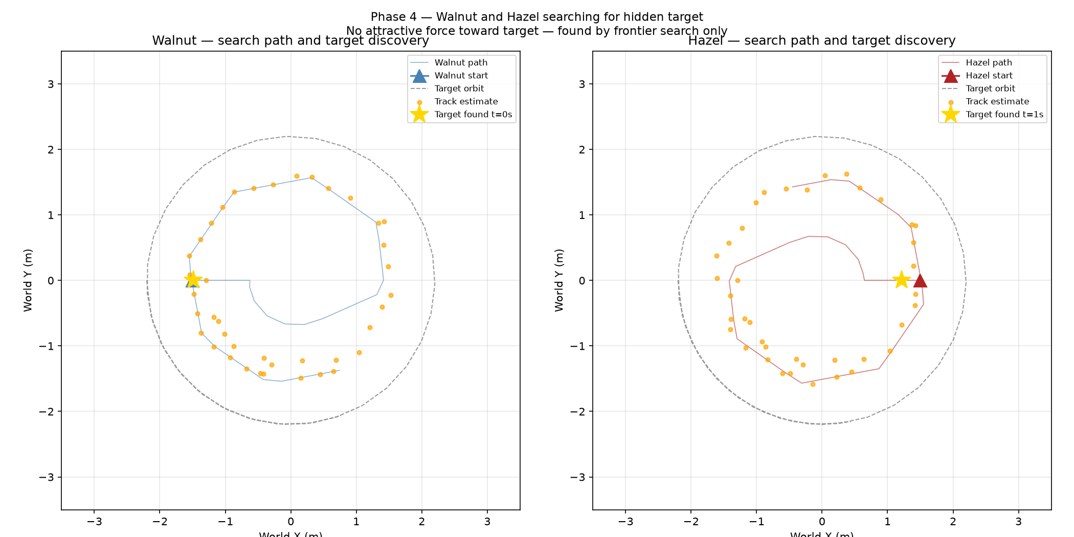
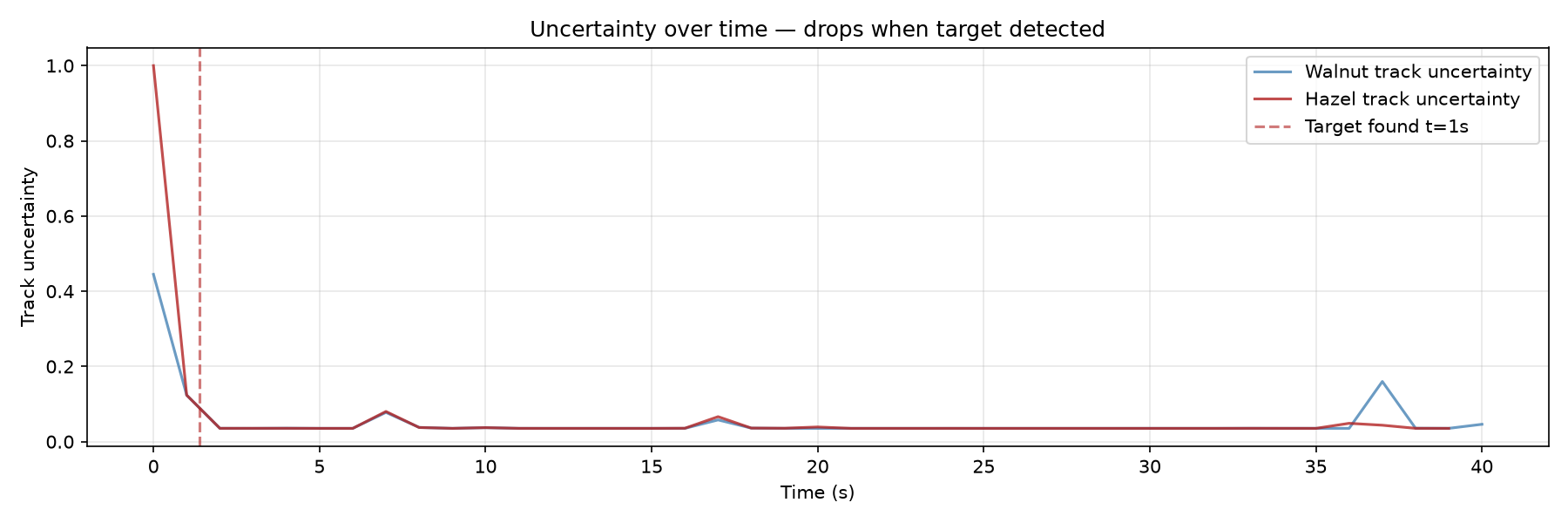
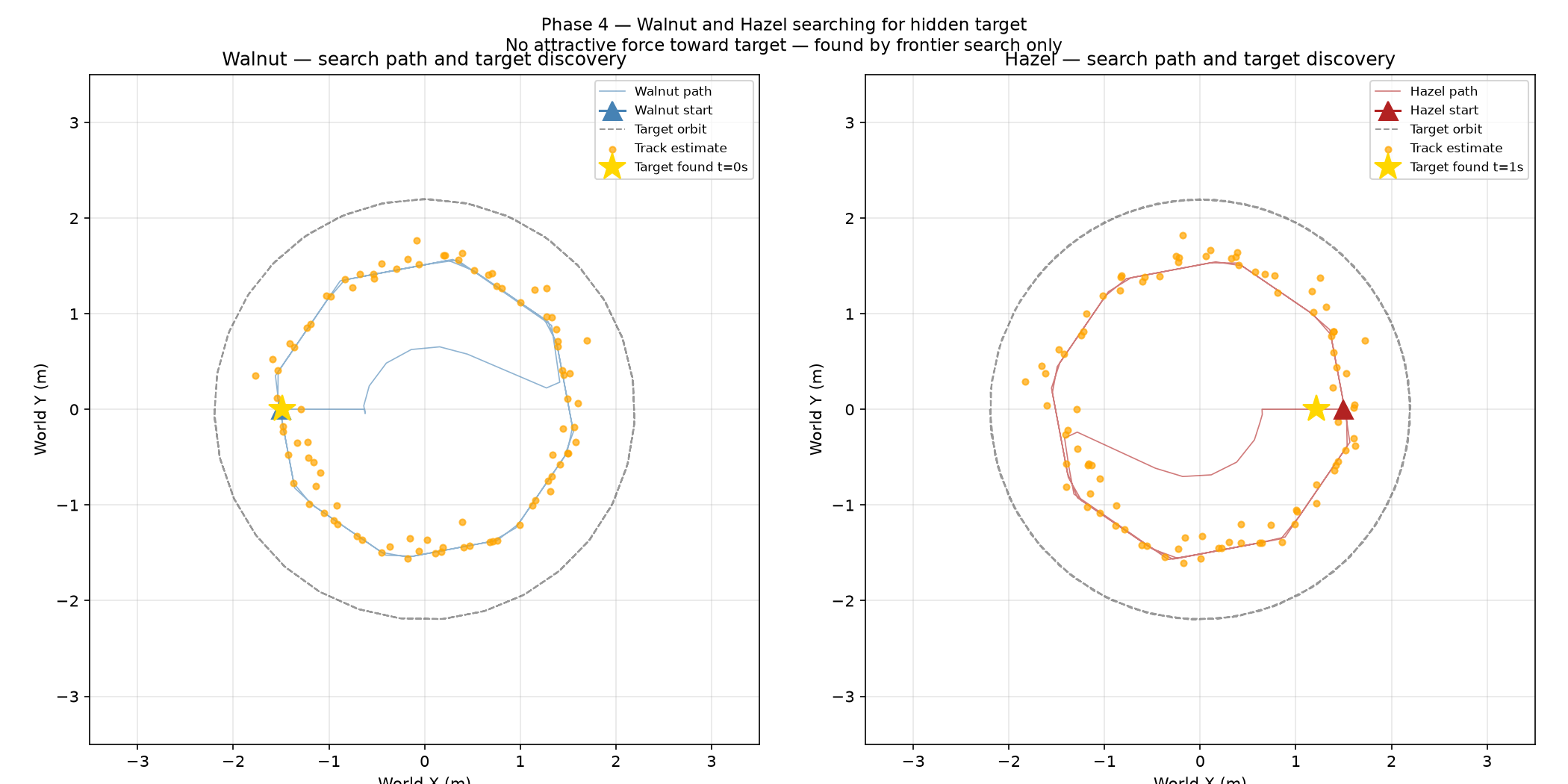
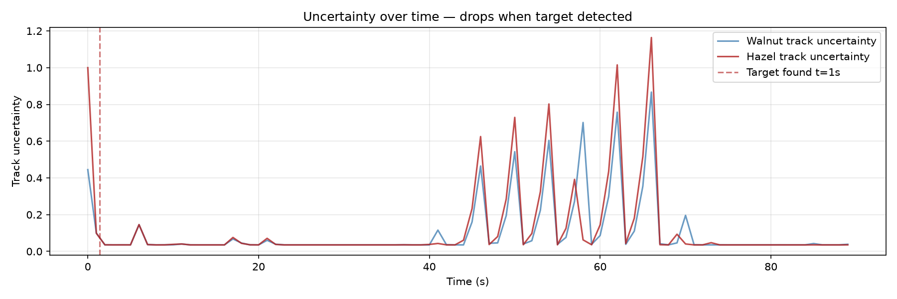
Phase 4b — A more complex world

Phase 4b makes the world more complex and more realistic:

A larger arena.
Internal obstacles.
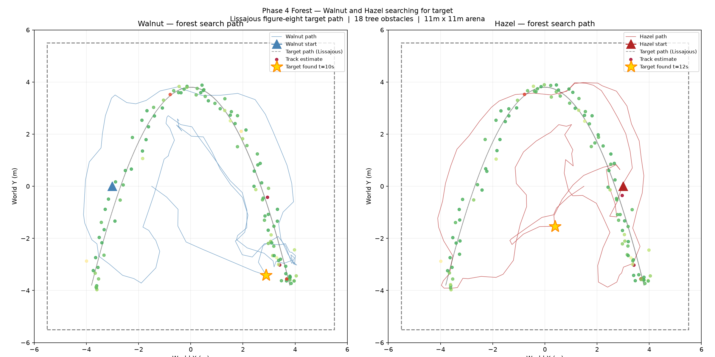
A more complex target path. This is a Lissajous curve, also called a figure-eight.

The three navigator classes

a. FrontierNavigator. This class selects unexplored grid cells as navigation targets.

The concept is correct. The implementation failed in practice. The pheromone grid starts empty. Therefore the frontier cells that the class selected were always next to the start position of the robot. The robot then oscillated between nearby cells. It never moved a useful distance. No code calls this class now.

b. WaypointNavigator. This class replaced FrontierNavigator. It does not depend on the grid. It visits a fixed circular set of waypoints.

c. APFNavigator. Both Phase 4 files use this class. It computes the velocity command from two sources:

The attractive force toward the current waypoint.
The repulsive forces from the obstacles.

This class is the actual motion controller. It handles obstacle avoidance.

A conceptual problem identified If the robots navigate between fixed waypoints in the arena, why does the pheromone grid exist? The robots must select their path from the pheromone grid.

In an unexplored environment there are no waypoints. The waypoint method therefore cannot work in the target application.

The peer position penalty

The peer position penalty, peer_pos, is a scoring modifier for the function find_farthest_frontier.

During the evaluation, the function checks each candidate cell. If a candidate cell is within 1.5 m of the position of the peer robot, the function multiplies its score by 0.3. The cell then becomes less attractive.

The robots did not move when the system used frontier-based navigation.

Root cause. The pheromone grid is a 12 m × 12 m sliding window. The window is centred on the robot. But the arena is only 11 m × 11 m.

Therefore a robot at (−3, 0) has grid cells from (−9, −6) to (3, 6). Approximately half of that grid is outside the arena walls.

The robot can never visit those out-of-arena cells. Therefore those cells keep $\mu = 0$ and $\sigma^2 = 1.0$ permanently. They are permanent frontiers.

The function _find_farthest_frontier selects the farthest frontier by design. Therefore it always selected an unreachable cell outside the walls.

Earlier debug output confirmed this, but the result was not noticed at the time. The goal returned as (5.875, −5.875). That position is outside the 5.5 m arena.

Effect. The robot moves toward an unreachable goal. It reaches the position clamp at ±5.0. It can never arrive. Therefore it never plans a new route to a reachable frontier.

The stuck-escape function of the APF navigator fires periodically. This produces the small y-axis movement in the logs: 0.09, −0.09, 0.16, −0.25. The frontier selection then immediately pulls the robot back to the wall.

Defect table

These six defects were found and corrected.

#	Symptom	Root cause	Correction
1	The robots stopped at ±3.3, then at ±5. They rotated without purpose in a corridor.	The walls were passed to the APF as circles with a radius of 5.5 m, centred on the midpoint of each wall. Their repulsion shells were rings that cut through the middle of the arena. The rings pushed the robots outward. Beyond \|x\| ≈ 4, the `0 < d` guard failed. The repulsion then disappeared completely.	The walls became four axis-aligned planes, through a `bounds` argument. The walls were removed from the obstacle list.
2	The mode stayed at `EXPLORING` permanently, even at the message `TARGET FOUND`.	The gate condition was `trace(P)/4 < 0.02`. That expression averages the position variance and the velocity variance. The velocity variance is approximately 26 times larger. Therefore the minimum possible value was 0.0658. The condition could never be true.	Gate on the position variance only. Add hysteresis: enter at 0.05, leave at 0.25.
3	The estimate moved instantly across the arena. Both robots reported the same incorrect data.	The `argmax` of the grid is a memory of a position where a detection occurred at some earlier time. The system supplied that value to the Kalman filter as a live measurement.	The grid now supplies a search goal, in the `INVESTIGATING` mode. The grid never supplies a measurement.
4	The estimates were biased toward the robots.	The distance was measured from the sensor ring, but reconstructed from the body centre. The result was 0.7 m short every time. Also, the code called `update()` once for each detecting ray. This collapsed the covariance matrix P.	Reconstruct the position from the sensor origin. Use the closest ray only.
5	Too many trees. The world formed a corridor.	The exclusion disks used old spawn points at (±3, 0) instead of the real spawn points at (±1.5, 0). This cut a 5 m clear channel and forced all 18 trees into two bands. Also, `d0 = 1.2` was larger than the gap between the trees. The robots could not pass between them.	Compute the clearance from the real spawn points. Set the spacing to 1.8 m and `d0` to 0.45.
6	Timing errors between the physics and the filters.	The physics loop and each agent kept separate clocks. None of those clocks matched wall time. At the same time, the function `predict()` used a hard-coded `dt = 1/240`.	Use one `SIM_CLOCK`, owned by the physics thread. The filter then integrates the real elapsed `dt`.

Two additions made during the correction work

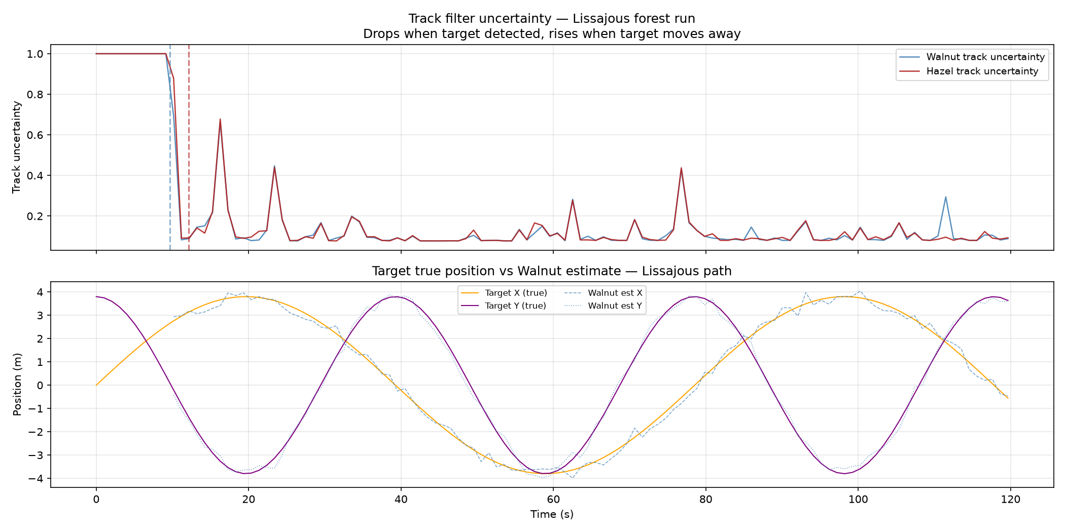
Track dropping after 8 seconds without a detection. The correction of defect 3 showed a new problem. A Kalman filter with no measurements diverges to approximately 10⁴. The stale grid data had concealed this behaviour.
Peer fusion gated on the confidence of the peer. This change also made the bootstrap branch in fuse_peer_track reachable for the first time.

Phase 4b results

Two plots side by side. Each shows an 11 by 11 metre arena with a dashed boundary, many green dots that mark tree obstacles, a figure-eight target path, and a robot path that moves around the obstacles. A yellow star marks the discovery position. — **Phase 4 forest — Walnut and Hazel search for the target.** The arena is 11 m × 11 m and contains 18 tree obstacles. The target follows a Lissajous figure-eight path, shown by the green points. The left plot shows the path of Walnut, who found the target at t = 10 s. The right plot shows the path of Hazel, who found the target at t = 12 s. Both robots move through the obstacle field without collisions, which confirms that the APF repulsion operates.

Two plots. The upper plot shows track filter uncertainty over 120 seconds. Both traces fall from 1.0 to near zero at about 12 seconds and stay low, with occasional small peaks. The lower plot shows the true target X and Y positions as smooth curves, with the Walnut estimates plotted on top of them. — **Phase 4 forest — track filter uncertainty and position tracking.** The upper plot shows that the uncertainty falls when the robots detect the target. The uncertainty rises when the target moves away. After the initial detection at approximately t = 12 s, both traces stay below 0.2 for most of the 120-second run. The lower plot compares the true target X and Y positions with the estimates of Walnut. The estimates follow the Lissajous path closely.

Phase 5 integrates the system and measures the results. Continue to Phase 5 and Phase 6 — Planned Work.

Phase 4 — Navigation and Search