Goal
Add the second robot, Hazel, and a communication protocol between the two robots.
When Walnut sees the target, Walnut broadcasts that information to Hazel. Hazel then updates her world model. Both robots act on shared knowledge. Neither robot has global information.
Why this phase is the core of the project Before this phase, the system was a robot with sensors. After this phase, the system is an actual swarm.
The decentralized architecture
The system is decentralized. There is no central coordinator. There is no shared memory. There are only messages between peers.
The simulation problem
Before this phase, one PyBullet world contained Walnut. This is no longer sufficient.
Hazel and Walnut run as two separate Python processes. Both processes must share the same physical PyBullet world. Two separate PyBullet instances cannot do this.
Solution. Start PyBullet in server mode. This creates one shared physics world. Both agents connect to that world as clients.
UDP sockets
UDP means User Datagram Protocol. UDP is a communication standard. It operates over any physical medium that connects the devices: Wi-Fi, Ethernet, or cellular.
In this simulation, both robots run on the same laptop. Therefore the network is the loopback interface at 127.0.0.1. The messages move through the networking stack of the operating system. The messages never touch a physical radio.
UDP is only a software protocol. It operates on top of the medium that carries the bits.
Other communication methods
The correct sensor type and the correct communication protocol depend on the range and on the environment.
For swarm communication without infrastructure, two methods exist:
- Delay-tolerant networking (DTN).
- Direct radio protocols. These protocols do not use IP. IP requires infrastructure. In a search and rescue situation, that infrastructure may not exist.
Research directions
Three open problems were identified for this phase.
Idea 1 — Stigmergic gradient fields instead of explicit messaging
The robots do not broadcast a statement such as “I think the target is at [x, y]”. Instead, each robot deposits a virtual pheromone gradient in a shared spatial map. The other robot then follows the gradient.
The new part is that this happens without shared memory. Each robot keeps its own gradient estimate. The robots reconcile the estimates with sparse messages that carry position stamps.
This method is closer to the operation of real ant colonies. The convergence properties under communication dropout are an open research question.
Idea 2 — Uncertainty-aware belief propagation
In the first design, Walnut detects the target and broadcasts a position estimate. That estimate has a confidence value that decreases linearly.
The more interesting version represents the target belief as a probability distribution. The distribution is a Gaussian over position. When peer estimates arrive, the system performs Bayesian fusion.
Example: Walnut states “target at [1.2, 0.8] ± 0.3 m”. Hazel states “target at [1.1, 0.9] ± 0.4 m”. Correct fusion produces an estimate that is tighter than either input.
This method has the name distributed Kalman filtering. Open questions remain about correct operation under asynchronous and lossy communication. Those are the exact conditions in a remote search and rescue scenario.
Idea 3 — Byzantine-resilient coordination
What happens if the sensors of one robot fail, and that robot broadcasts incorrect target positions?
In the current protocol, Hazel adopts the incorrect estimate of Walnut without any check.
Byzantine fault tolerance in small swarms of two to four agents, under resource constraints, is not well studied. A possible implementation is a simple reputation system. The system weights peer estimates by their historical accuracy. You can then measure how quickly the swarm recovers from a faulty agent.
The chosen direction
Decision Pursue a combination of Idea 1 and Idea 2.
Stigmergy solves the problem “where do we look”. Bayesian fusion solves the problem “how confident am I”.
The combination may be novel. It is a distributed pheromone field. Each cell carries a Gaussian belief, which is a mean and a variance, instead of a scalar intensity. The system fuses the cells with a Bayesian update when peer grid patches arrive over lossy communication.
The novelty has two parts:
- A shared spatial map without shared memory. Each robot keeps its own estimates.
- The combination of the two ideas.
Stigmergy — uncertainty-aware navigation
In ant colonies, the ants do not know the position of the food. The ants move at random.
When one ant finds food, that ant deposits a pheromone trail on its way home. Other ants follow the trail and make the trail stronger. Shorter paths become stronger faster, because the ants return sooner.
Over time, the colony converges on the shortest path to the food. No individual ant ever knows the global map.
The equivalent in this project. The pheromone is the probability grid. The grid is a two-dimensional map. Each cell holds a belief about the presence of the target in that cell. The belief has both a mean and a variance.
The robots deposit belief when their sensors fire. The robots then follow the gradient toward a higher belief. The gradient is the digital equivalent of the pheromone trail.
Why the original design was not sufficient
Original plan. Walnut broadcasts target information over UDP. Walnut and Hazel then move to the target.
Problems with that plan:
| Problem | Effect |
|---|---|
| The target moves | The information becomes stale |
| Communication fails, for example in a dense forest, in rubble, or with interference | The information becomes stale, or the robot cannot trust it |
| Observations conflict | Which information do you accept? |
Solution. Stigmergy and distributed Kalman filtering.
The Kalman filter from first principles
Rudolf Kalman invented the Kalman filter in 1960. It is one of the most important algorithms in engineering. It operates in every GPS receiver, every aircraft autopilot, every missile guidance system, and every self-driving car.
The problem that it solves
You want to know the true state of something. The state can be a position, a velocity, a temperature, or any other quantity.
You have two sources of information:
- A model of how the state changes over time.
- Measurements that contain noise.
Neither source is completely reliable. The Kalman filter states how to combine the two sources in the optimal way.
The key concept
Your prediction and your measurement are both Gaussian distributions. They are not point estimates.
The filter does not hold the statement “the state is X”. The filter holds the statement “the state is probably X, with uncertainty $\sigma^2$”. The filter updates this belief at each step.
Why the distribution is Gaussian
Gaussian distributions have one important property. The product of two Gaussians is another Gaussian.
Therefore, when you fuse two uncertain estimates, you always get one clean uncertain estimate. No other family of distributions has this property in closed form.
The two-step cycle
PREDICT step — time passes, uncertainty increases
─────────────────────────────────────────────────
The state changes according to your motion model.
Your last measurement may have been perfect. But the world
has moved since then. Therefore you are less certain now.

mu_pred     = F × mu             F = state transition matrix
                                 (how the state changes without control input)
sigma²_pred = F² × sigma² + Q    Q = process noise
                                 (how much the uncertainty grows per timestep)

UPDATE step — a new measurement arrives, uncertainty decreases
──────────────────────────────────────────────────────────────
A sensor reading is a noisy observation of the true state.
Use it to move your prediction toward the truth.

K           = sigma²_pred / (sigma²_pred + R)   Kalman gain
                                                R = measurement noise
mu_new      = mu_pred + K × (z − mu_pred)       z = measurement
sigma²_new  = (1 − K) × sigma²_pred
The Kalman gain
The Kalman gain $K$ is the central part of the filter. Its value is between 0 and 1. It answers one question: how much must I trust this measurement, compared with my prediction?
| Condition | Result | Effect |
|---|---|---|
| $R$ is large (noisy sensor) | $K$ is small | Trust the prediction more |
| $\sigma^2_{\text{pred}}$ is large (uncertain prediction) | $K$ is large | Trust the measurement more |
| $R \approx \sigma^2_{\text{pred}}$ | $K \approx 0.5$ | Weight both equally |
This result is optimal. It minimizes the mean squared error, under the assumption of Gaussian noise. No other linear estimator gives a better result.
With a control input
The predict step can also include a control input:
mu_pred     = A × mu + B × u        (where did we expect the target to move?)
sigma²_pred = A² × sigma² + Q       (uncertainty increases with time — process noise Q)
The relation to the product of Gaussians
Important relation The update step of the Kalman filter is the product of two Gaussians.
The product of Gaussians performs the update step without the predict step. This is acceptable if the target does not move. In this project, the target does move. Therefore the predict step is necessary.
Each cell in the grid runs its own one-dimensional Kalman filter. Each cell tracks:
- The probability that the target is in that cell. This is the predict step.
- A motion model. Neighbouring cells share probability, because the target may move there.
- The measurement, which is the infrared sensor reading.
Distributed Kalman filtering
A distributed Kalman filter has multiple agents. Each agent has partial measurements. Each agent keeps its own belief. The agents share beliefs with peers from time to time.
In its full form, the distributed Kalman filter assumes linear Gaussian dynamics. It also requires the solution of a Riccati equation at each fusion step.
The distributed part
Neither Walnut nor Hazel has all of the measurements. The robots never share raw sensor readings. The robots share only their current belief state, which is $(\mu, \sigma^2)$. The distributed Kalman filter then fuses these beliefs.
# Walnut's belief about cell (i,j): (mu_W, sigma²_W)
# Hazel's belief about cell (i,j):  (mu_H, sigma²_H)
# These are independent estimates of the same quantity.

# Information form fusion.
# This IS distributed Kalman filtering, not only a product of Gaussians:
information_W = 1 / sigma²_W          # Walnut's certainty
information_H = 1 / sigma²_H          # Hazel's certainty

fused_info    = information_W + information_H
fused_sigma²  = 1 / fused_info        # the combined certainty is always higher
fused_mu      = fused_sigma² * (information_W * mu_W + information_H * mu_H)
Three challenges
| Challenge | Description | Solution |
|---|---|---|
| Double counting | Also called the rumour propagation problem. Shared information is counted more than once. | Covariance intersection |
| Communication delays | Messages arrive after the state has changed. | Timestamp each belief |
| Asynchrony | The beliefs are never at the same timestep. The standard Kalman filter assumes synchronous measurements. | Apply a staleness penalty |
Covariance intersection
Why it is necessary
Naive fusion, which is the product of Gaussians above, assumes that the estimate of Walnut and the estimate of Hazel are independent.
They are not independent. The robots have exchanged messages. The current belief of Walnut already includes information that Hazel sent earlier.
If you fuse the estimates as independent estimates, you count that shared information twice. The result is falsely confident.
The method
Covariance intersection (CI) is a conservative fusion rule. It stays correct for any correlation between the estimates. Julier and Uhlmann introduced the method in 1997. It is the standard approach in multi-robot estimation.
# omega ∈ [0,1] is optimized to minimize the trace of the fused covariance.

fused_sigma²_inv = omega / sigma²_W + (1 − omega) / sigma²_H
fused_sigma²     = 1 / fused_sigma²_inv

fused_mu = fused_sigma² * (omega * mu_W / sigma²_W
                         + (1 − omega) * mu_H / sigma²_H)

# The optimal omega minimizes fused_sigma², which maximizes the certainty.
# For the scalar case:  omega = sigma²_H / (sigma²_W + sigma²_H)
When $\omega = \sigma^2_H / (\sigma^2_W + \sigma^2_H)$, the formula becomes a weighted average. The weighted average gives more weight to the more confident estimate.
The resulting fused_sigma² is always larger, and therefore more conservative, than the
naive product of Gaussians. Covariance intersection never claims certainty that the
system does not have.
Design questions and answers
Three engineering questions were raised before the code was written.
Question 1 — Does the spatial map grow? Is the memory use efficient?
In the simple implementation, yes, the map grows. The grid would be a fixed size that covers the whole arena. This wastes memory on cells that are far from both robots. Those cells will never be relevant.
For a small arena of 5 m × 5 m, this is not a problem. For a real deployment over a football field or a forest, it is a problem.
The correct solution is a sliding window grid. Each robot keeps a fixed-size grid, for example 50 × 50 cells. The grid is centred on the current position of that robot. When the robot moves, the grid moves with it. Cells that leave the window are removed. New cells that enter the window are initialized with maximum uncertainty, which is $\mu = 0$ and a large $\sigma^2$.
This gives O(1) memory use, independent of the arena size. This is the correct complexity for a deployed system.
One complication. When two robots share grid patches, the patches are in different reference frames. Each grid is centred on its own robot. Therefore the patch must carry world-frame coordinates for each cell. The receiver then places the cells correctly in its own local grid.
This is also more realistic. Real robots do not share a coordinate system by default. Real robots must establish one.
Each grid patch message includes the world-frame origin of the grid of the sender. The receiver then performs the coordinate mapping.
Question 2 — Is this still without shared memory?
Yes. This point is important, because it is the core architectural claim.
In distributed systems, “shared memory” means a memory region that several processes can read and write directly. It is like a global variable that all processes can access.
This is what shared memory would look like. This project does not do this:
# SHARED MEMORY approach — NOT used in this project
global_grid = SharedGrid()   # exists where both robots can access it
walnut.update(global_grid)   # both write to the same object
hazel.update(global_grid)
That design is centralized. It fails if the shared memory server fails. It does not scale to robots on separate physical machines. Real swarms do not operate in this way.
This is what the project does:
# DISTRIBUTED approach — used in this project
walnut_grid = PheromoneGrid()   # exists only in Walnut's process memory
hazel_grid  = PheromoneGrid()   # exists only in Hazel's process memory

# Synchronization occurs ONLY through UDP messages.
# Neither robot can read the grid of the other robot directly.
# Each robot can only infer the beliefs of the other from received patches.
Each robot owns its grid exclusively. Beliefs move between robots only through UDP messages that contain grid patches.
If the network fails, each robot continues with its own local grid. The beliefs then diverge. This is the correct behaviour for a decentralized system. The beliefs converge again when communication returns.
One clarification about PyBullet
The PyBullet shared memory option, p.SHARED_MEMORY, is only for the physics
simulation. It is how both processes access the same simulated world, which includes the
robot positions and the joint states.
This is a simulation artifact. It is not part of the swarm architecture. In a real deployment there is no PyBullet. Each robot has its own sensors and its own actuators. The physics server does not exist. Only the communication protocol remains.
The explicit claim. Two robots, each with private memory, build a shared understanding of the world. They do this only through sparse, timestamped UDP messages that carry partial grid patches. There is no shared memory. There is no central server. There is no global state.
Question 3 — Is timestamping necessary, or is it too expensive?
Timestamping is completely necessary. This example shows why:
t=0.0s  Walnut detects the target at [1.2, 0.8]. Walnut deposits a high mu there.
t=0.1s  Walnut broadcasts the grid patch to Hazel.
t=0.5s  Hazel receives the patch. The packet was delayed in a queue.
t=0.5s  By this time, the target has moved to [1.8, 0.3].
Without timestamps, Hazel fuses the observation from t = 0.0 s as a current observation. Hazel then searches [1.2, 0.8], but the target is already at [1.8, 0.3]. An older message produces a larger error.
With timestamps, Hazel knows that the patch is 0.5 seconds old. Hazel can then apply a staleness penalty before fusion. The penalty increases the $\sigma^2$ of the received cells in proportion to their age.
Old information is still useful. The target has probably not moved far. But the system treats old information as less certain. This is the same operation as the predict step in the Kalman filter: uncertainty increases with time, because the target moves.
The computational cost is almost zero. The system attaches one float to each message. It then performs one multiplication per cell during fusion.
An expensive version also exists. That version rolls beliefs back to match the timestamps. It requires storage of the full history of the belief trajectory of each cell. This project does not need that version.
The lightweight version applies a staleness factor to $\sigma^2$. It gives approximately 95 % of the benefit at almost no cost:
# On receipt of a patch with timestamp t_sent, at current time t_now
staleness    = t_now - t_sent            # age in seconds
sigma²_stale = sigma²_received + Q_drift * staleness
# Q_drift = how much the uncertainty grows per second (tunable)
# Fuse sigma²_stale instead of sigma²_received.
This costs one float per received patch. The overhead is negligible. The improvement in correctness is significant.
The architecture
Per-cell pipeline at each timestep
1. PREDICT:  mu_pred     = mu + diffusion_from_neighbors
             sigma²_pred = sigma²_pred + Q   (uncertainty grows — the target may move)

2. UPDATE (only if a sensor hit occurred in this cell):
             K           = sigma²_pred / (sigma²_pred + R)
             mu_new      = mu_pred + K × (z − mu_pred)
             sigma²_new  = (1 − K) × sigma²_pred

3. DECAY:    mu_new     *= (1 − decay_rate)   (the pheromone evaporates)

4. FUSE (only when a peer grid patch arrives):
             Use the information filter formula above.
The complete revised architecture
Each robot keeps:
  PheromoneGrid:
    - A fixed W×H sliding window, centred on the robot's current position
    - Each cell holds (mu, sigma²) in world-frame coordinates
    - Memory: O(W×H), constant for any arena size
    - Edges: cells that leave the window are removed; cells that enter
             are initialized to (0, sigma²_max)

At each timestep:
  1. SLIDE      Shift the grid if the robot has moved significantly.
  2. PREDICT    Diffuse mu to the neighbours. Add Q to every sigma².
  3. DEPOSIT    Run the Kalman update on cells where the IR sensor hit the target.
  4. DECAY      mu *= (1 − decay).  sigma² += decay_noise.
  5. FUSE       On receipt of a peer patch:
                  apply the staleness penalty to the received sigma²
                  run covariance intersection on each overlapping cell
  6. BROADCAST  Every N steps, send a sparse patch of the cells where mu > threshold.
                Include: world-frame cell coordinates, mu, sigma², timestamp.

Communication:
  - No shared memory
  - UDP only
  - Each patch is self-contained, with world coordinates and a timestamp
  - The receiver maps the received cells into its own local grid frame
Personal note Concepts learned so far: the sliding window; the world coordinate system and the local coordinate system may differ, so cells cannot be updated correctly without a conversion; Gaussian distributions; statistics.
The limitation, and the second filter layer
Limitation found. Independent grid cells cannot learn trajectories. Therefore the uncertainty returns to 100 % when the target leaves sensor range. A better estimate requires track maintenance.
Solution. Add a five-step Kalman filter above the pheromone layer. Its function is to track the target. It maintains a belief about the position of the target at the present moment.
The two layers
| Layer | Component | Function |
|---|---|---|
| Layer 1 | Pheromone grid, with a Kalman filter in each cell | Spatial memory of the detection history |
| Layer 2 | Four-state track filter | A persistent belief about the position and the velocity of the target |
Results
Uncertainty comparison
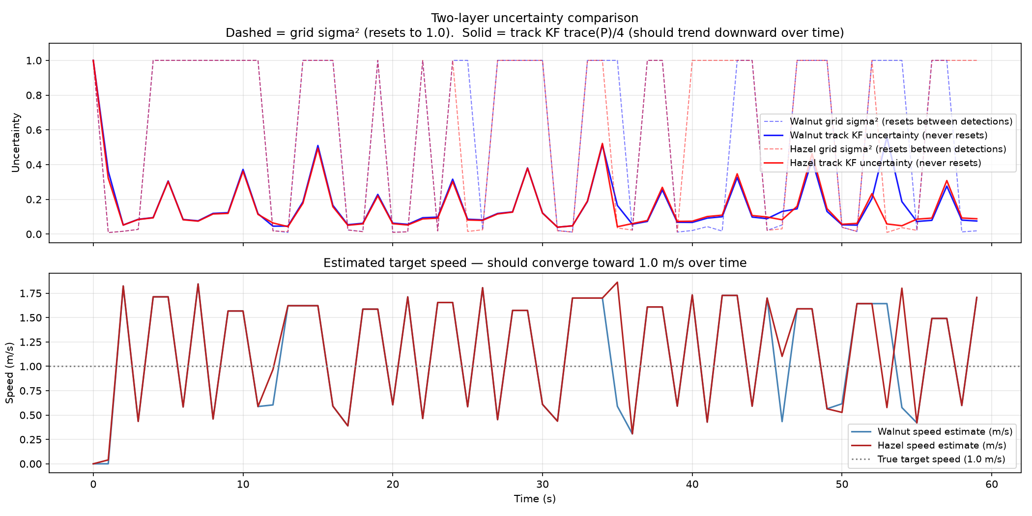
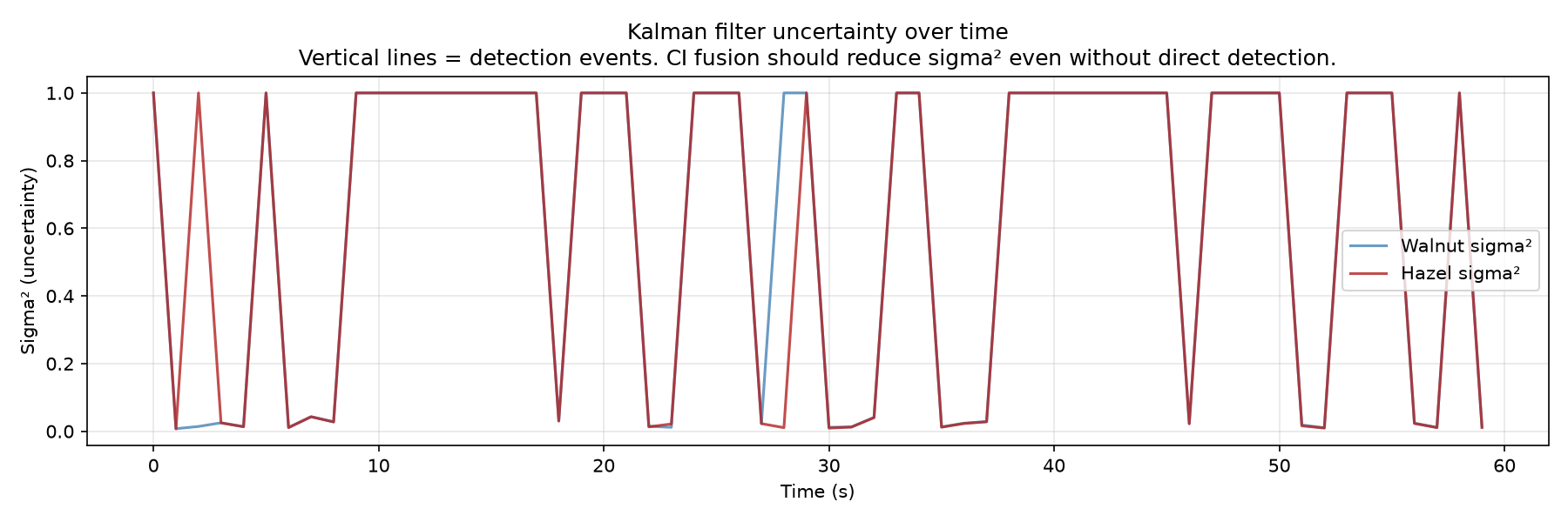
The dashed lines show the grid $\sigma^2$. These lines still increase to 1.0 between detections, as before.
The solid lines show the track filter, as $\text{trace}(P)/4$. These lines behave completely differently. They never return to 1.0. After the first detections near t = 2 s, the solid lines stay below 0.5 for the rest of the run. From t = 20 s onward, they stay in the range 0.05 to 0.15, with small oscillations.
This downward trend in the first 20 seconds, and then the stable low uncertainty, is the intended learning behaviour. The filter has learned the motion of the target. It now maintains persistent confidence.
Speed estimation
The true target speed is 1.0 m/s, shown as the dotted line.
The estimates oscillate between 0.4 and 1.8 m/s. They do not converge cleanly to 1.0 m/s. This is expected.
The reason is as follows. The track filter receives only position measurements, from infrared detections. The target passes through the sensor range of each robot for a short time only. Between detections, the velocity estimate drifts. The filter predicts from a position that the target has already left.
The speed estimate is most accurate immediately after a detection. The logs show
v=0.97m/s and v=1.10m/s at the moments of direct detection. The estimate then
degrades between detections.
This is a fundamental limit of sparse observations. The velocity estimate is noisy. The position estimate stays good, because frequent fusions anchor it.
Trajectories
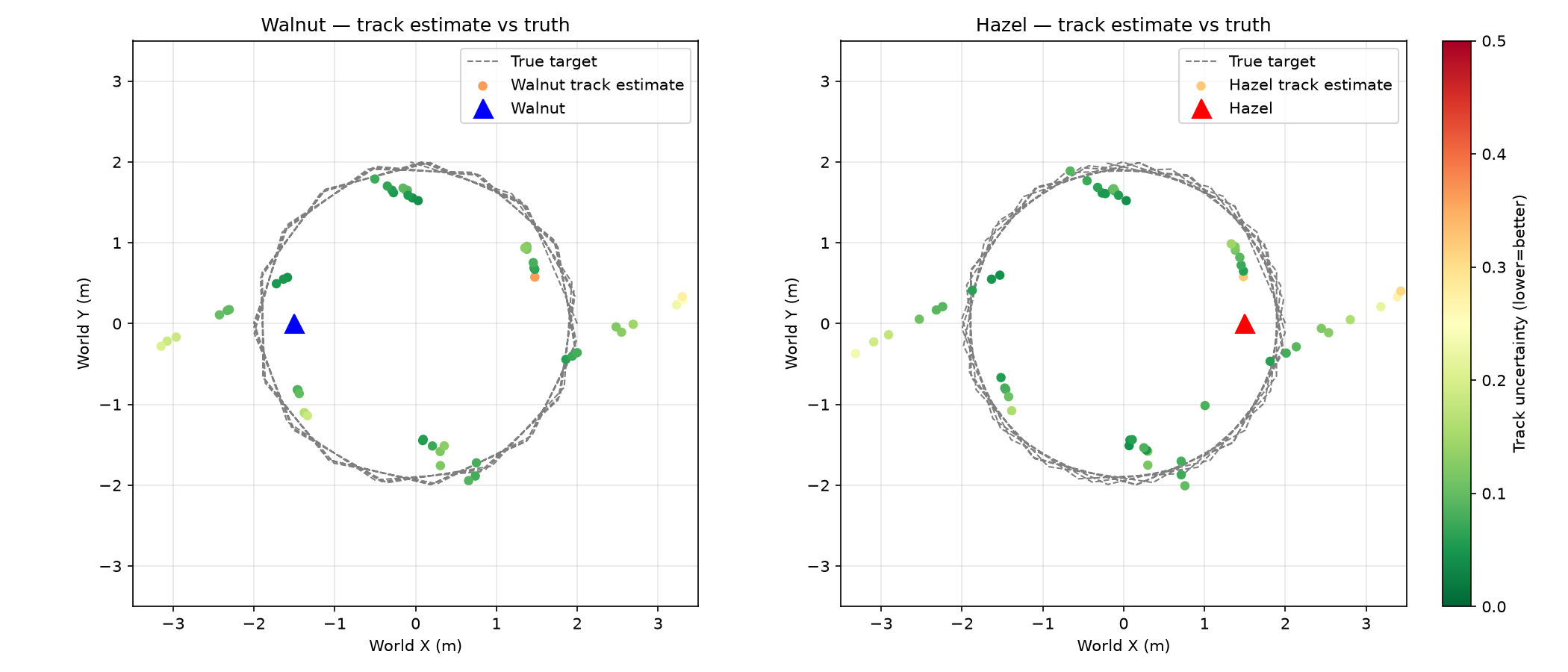
The estimate points are now mostly dark green. This means low uncertainty, near 0.0 to 0.1. The points sit tightly on the orbital arc.
This is a large improvement over the earlier runs, where all points were yellow. The track filter now produces confident and accurate estimates.
Some points appear slightly inside or outside the arc. These are the predictions between detections, where the filter propagates the velocity estimate forward.
Estimation error
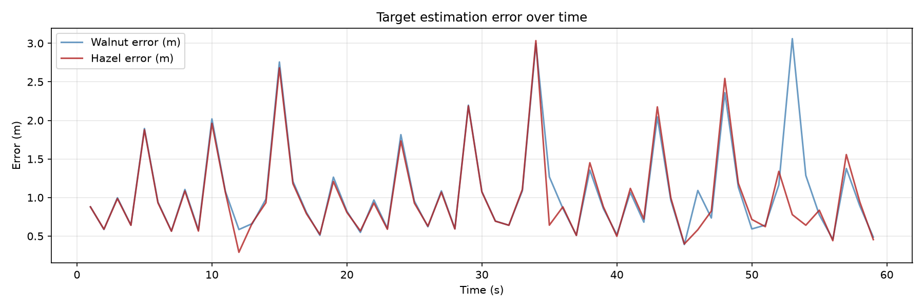
The error oscillates between 0.4 m and 3.0 m.
The peaks, at 2.0 to 3.0 m, occur when the track filter has predicted without a detection for several seconds. The target has then moved a significant distance from its last known position.
The minima, at 0.4 to 0.6 m, occur immediately after a detection.
The error does not decrease continuously, because the target continues to move. This is the correct behaviour for a reactive tracker. It is not a failure.
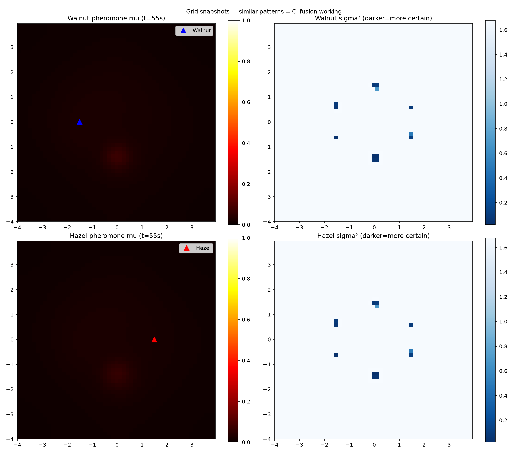
Grid snapshots
Both $\mu$ grids now show a faint red region near the lower-left area. This is where the target is at approximately t = 55 s. Earlier runs showed only black.
More importantly, the $\sigma^2$ panel of Walnut and the $\sigma^2$ panel of Hazel are almost identical. This occurs although the robots are on opposite sides of the arena. The dark blue cells, which are confident and have a low $\sigma^2$, appear at the same world positions in both grids.
This confirms that the spatial covariance intersection fusion operates. Walnut has a low $\sigma^2$ at positions that Hazel detected, and Hazel has a low $\sigma^2$ at positions that Walnut detected.
Log values
| Value | Reading | Meaning |
|---|---|---|
n_updates |
Above 600 for each robot | The track filter received more than 600 measurement updates in 60 seconds. Most updates come from the confident best estimate of the grid, which feeds the track filter between direct detections. This is the if not detected: grid_est → track.update() path. The two-layer architecture operates as designed: the grid collects spatial evidence, and the track filter consumes that evidence continuously. |
fusions |
Increases from 0 to 10 | Cross-robot covariance intersection fusions occur at both the grid level and the track level. The rate increases in the second half of the run, because both robots then have more patches to share. |
Walnut sent=600 recv=599 |
One lost packet in 60 seconds | This is 99.8 % delivery on loopback UDP. With a real radio, delivery would be 70 % to 90 %. The covariance intersection fusion would then degrade gracefully. |
| Speed at detection | v=0.97m/s at t = 12 s (Hazel), v=1.10m/s at t = 46 s (Hazel) |
These are the two direct infrared detections in the logs. Both produce speed estimates within 10 % of the true 1.0 m/s. The filter is accurate at the moment of observation. |
Phase 3 summary
Layer 1 — the pheromone grid with a Kalman filter in each cell. This is the spatial memory of the detection history. Each cell carries $(\mu, \sigma^2)$. The grid deposits, diffuses, and decays. Covariance intersection fuses the grid when patches arrive. The novel element is the per-cell Gaussian belief in a stigmergic field.
Layer 2 — the four-state track filter. This is a persistent belief about the position and the velocity of the target. It never resets. The predict step propagates the belief forward with the velocity estimate. The update step fuses measurements from the sensors and from the grid. Matrix covariance intersection fuses the 4 × 4 covariance.
Distributed communication. 600 UDP messages per robot. No shared memory. Sparse patches. Timestamps for staleness handling. Covariance intersection prevents overconfidence during repeated information exchange.
Quantitative results. The track uncertainty stabilizes below 0.15 after 20 seconds. The speed estimates reach within 10 % of the true value at the moments of detection. Both robots agree on the same spatial positions, although they have no shared memory.
What the phase must prove
- Fusion improves accuracy. Compare the individual $\mu$ grid of each robot, the fused grid, and the true target position.
- Covariance intersection operates correctly.
- Stigmergy produces emergent coverage. The two robots avoid the same areas without a programmed avoidance rule.
- The system degrades gracefully under packet loss.
Next
Phase 4 adds navigation and obstacle avoidance. Continue to Phase 4 — Navigation and Search.